In order to understand how to use this program, you need to consider EXCEL formulas with examples.
If you place the mouse cursor on any cell and click on the “select function” item, the function wizard appears.
With its help, you can find the necessary formula as quickly as possible. To do this, you can enter its name, use the category.

Excel is very convenient and easy to use. All functions are divided into categories. If the category of the required function is known, then its selection is carried out according to it.
If the function is unknown to the user, then he can set the category "full alphabetical list".
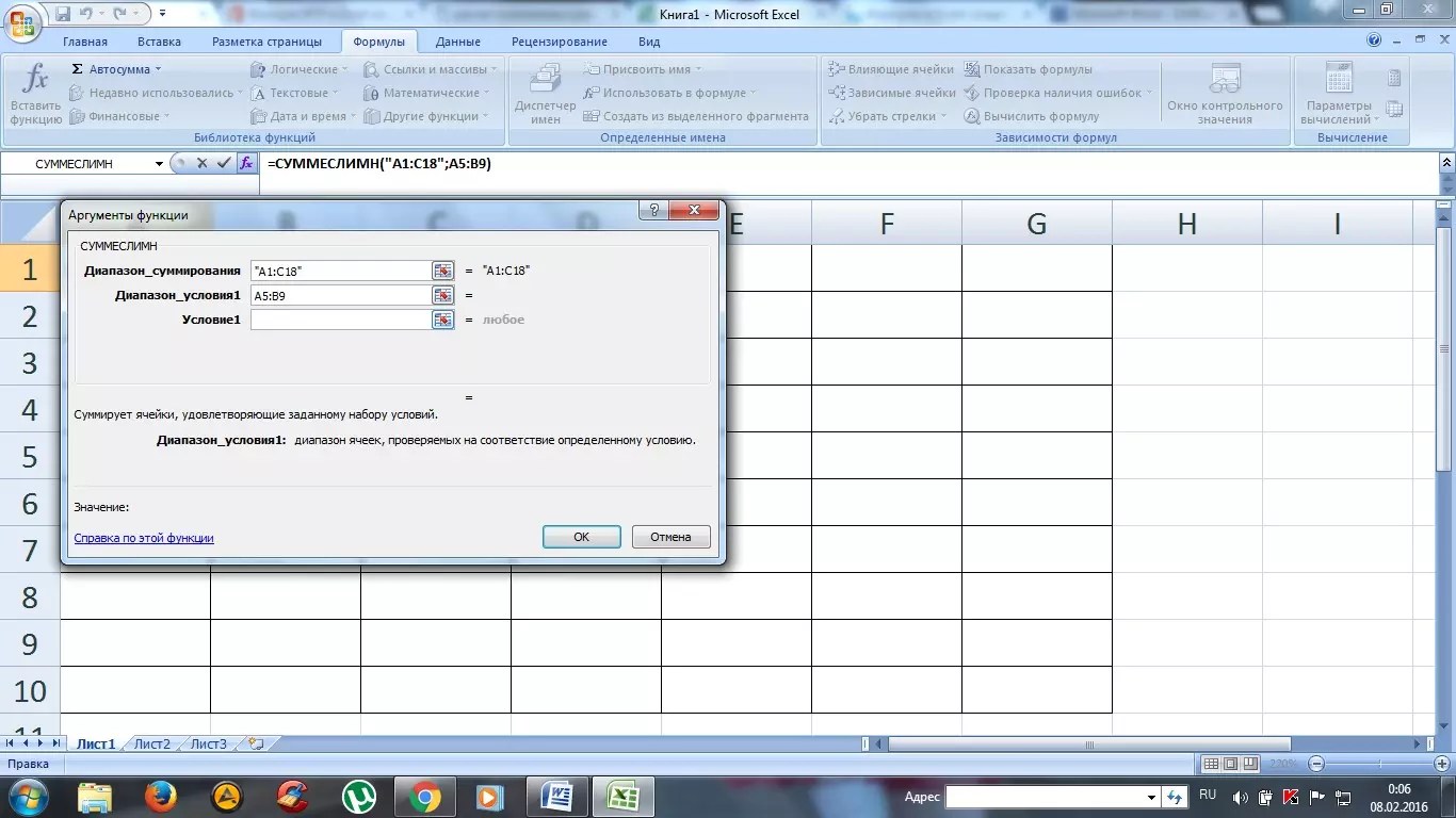
For example, given the task, find the function SUMIFS. To do this, go to the category of mathematical functions and find the one you need there.
VLOOKUP function
Using the VLOOKUP function, you can extract the necessary information from the tables. The essence of vertical lookup is to look for the value in the leftmost column of the given range.
After that, the total value is returned from the cell, which is located at the intersection of the selected row and column.
The calculation of the VLOOKUP can be seen in an example that shows a list of surnames. The task is to find the last name by the given number.

Applying the VLOOKUP function
The formula shows that the first argument of the function is cell C1.
The second argument A1:B10 is the range to search.
The third argument is the index number of the column from which to return the result.

Calculating a given last name using the VLOOKUP function
In addition, you can search for a last name even if some sequence numbers skipped.
If you try to find the last name from a non-existent number, the formula will not give an error, but will give the correct result.

Search for a last name with missing numbers
This phenomenon is explained by the fact that the VLOOKUP function has a fourth argument, with which you can set the interval view.
It has only two values - "false" or "true". If no argument is given, it defaults to true.
Rounding Numbers with Functions
The functions of the program allow you to accurately round any fractional number up or down.
And the resulting value can be used in calculations in other formulas.
The number is rounded using the ROUNDUP formula. To do this, you need to fill in the cell.
The first argument is 76.375 and the second is 0.

Rounding a number with a formula
In this case, the number has been rounded up. To round a value down, select the ROUNDDOWN function.
Rounding occurs to an integer. In our case, up to 77 or 76.
AT Excel program help simplify any calculations. With the help of a spreadsheet, you can complete tasks in higher mathematics.
The program is most actively used by designers, entrepreneurs, as well as students.
The whole truth about Microsoft Excel 2007 formulas
EXCEL formulas with examples - Instructions for use
A complex formula contains more than one operator compared to a simple formula such as 5+2*8. If a formula contains multiple mathematical operators, Excel follows the order in which it performs the calculation. When using Excel to calculate complex formulas, you need to know the order of operations:
- Expressions placed in brackets;
- Exponentiation (for example, 4^2);
- Multiplication and division, which comes first;
- Addition and subtraction, which comes first.
Create a complex formula
In the example below, I'll show you how Excel calculates complex formulas based on the order in which the operations are performed. AT this example Calculate the amount of sales tax for food services. To do this, write the following expression in cell D4: =(D2+D3)*0.075. This formula will add the value of all invoice items and then multiply by the 7.5% sales tax (written as 0.075).
As mentioned above, Excel follows the order of operations and first adds the values in brackets: (44.85+39.90)=$84.75. Then he multiplies this number by the tax rate: $84.75*0.075. The result of the calculation shows that the sales tax will be $6.36 .

Built-in Functions
Excel has functions for all occasions. Their use is necessary for solving various problems at work, study, etc. Some of them can be used only once, while others may not be needed. But there are a number of features that are used regularly.
If you select the “formulas” section in the main menu, then all known functions are concentrated here, including financial, engineering, and analytical ones. In order to select, you should select the item “insert function” or using the combination Shift+F3.

If you place the mouse cursor on any cell and click on the “Insert function” item, the function wizard appears. With its help, you can find the necessary formula as quickly as possible. To do this, you can enter its name or use the category.
Excel is necessary in cases where you need to organize, process and save a lot of information. It will help automate calculations, make them easier and more reliable. Formulas in Excel allow you to carry out arbitrarily complex calculations and get results instantly.
How to write a formula in Excel
Before learning this, you should understand a few basic principles.
- Each starts with an "=" sign.
- Values from cells and functions can participate in calculations.
- Operators are used as the mathematical signs of operations that are familiar to us.
- When you insert an entry, the default cell reflects the result of the calculation.
- You can see the design in the row above the table.
Each cell in Excel is an indivisible unit with its own identifier (address), which is denoted by a letter (column number) and a number (row number). The address is displayed in the field above the table.
So, how to create and insert a formula in Excel? Proceed according to the following algorithm:

Designation Meaning
Addition
- Subtraction
/ Division
* Multiplication
If you need to specify a number, not a cell address, enter it from the keyboard. To enter a negative sign in an Excel formula, press "-". 
How to enter and copy formulas in Excel
They are always entered after pressing "=". But what if there are many similar calculations? In this case, you can specify one, and then just copy it. To do this, enter the formula, and then "stretch" it in the right direction to multiply.
Set the pointer to the copied cell and move the mouse pointer to the lower right corner (on the square). It should take the form of a simple cross with equal sides. 
Click left button and pull. 
Release when you want to stop copying. At this point, the calculation results will appear. 
You can also stretch to the right.
Move the pointer to the next cell. You will see the same entry, but with different addresses. 
When copying in this way, the line numbers increase if the shift is down, or the column numbers increase if to the right. This is called relative addressing.
Let's enter the value of VAT into the table and calculate the price with tax. 
The price with VAT is calculated as the price*(1+VAT). Enter the sequence in the first cell. 
Let's try to copy the record. 
The result is strange. 
Let's check the content in the second cell. 
As you can see, when copying, not only the price shifted, but also VAT. And we need this cell to remain fixed. Fix it with absolute link. To do this, move the pointer to the first cell and click on the address B2 in the formula bar. 
Press F4. The address will be diluted with a "$" sign. This is the sign of an absolutely cell. 
Now after copying the address B2 will remain unchanged.
If you accidentally entered data in the wrong cell, just transfer it. To do this, move the mouse pointer over any border, wait until the mouse looks like a cross with arrows, press the left button and drag. AT right place just release the manipulator.
Using Functions for Calculations
Excel offers a large number of functions that are categorized. You can view the full list by clicking on the Fx button next to the formula bar or by opening the "Formulas" section on the toolbar. 
Let's talk about some of the features.
How to Set "If" Formulas in Excel
This function allows you to set a condition and perform a calculation depending on whether it is true or false. For example, if the quantity sold is more than 4 packs, more should be purchased.
To insert the result depending on the condition, let's add one more column to the table. 
In the first cell under the heading of this column, set the pointer and click the "Logical" item on the toolbar. Let's select the "If" function. 
As with inserting any function, a window will open to fill in the arguments. 
Let's specify a condition. To do this, click on the first row and select the first cell "Sold". Next, put the sign ">" and indicate the number 4. 
In the second line we will write "Purchase". This inscription will appear for those products that have been sold out. The last line can be left blank, since we have no action if the condition is false. 
Click OK and copy the entry for the entire column. 
So that the cell does not display "FALSE", open the function again and fix it. Place the pointer on the first cell and press Fx next to the formula bar. Insert the cursor on the third line and put a space between the quotation marks. 
Then OK and copy again. 
Now we see which product should be purchased.
formula text in excel
This feature allows you to apply a format to the contents of a cell. In this case, any data type is converted to text, and therefore cannot be used for further calculations. Let's add a column to format the total. 
In the first cell, enter a function (the "Text" button in the "Formulas" section). 
In the arguments window, specify a link to the cell of the total amount and set the format to "#RUB". 
Click OK and copy. 
If we try to use this amount in calculations, we will get an error message. 
"VALUE" means that calculations cannot be made.
You can see examples of formats in the screenshot. 
Date Formula in Excel
Excel provides many options for working with dates. One of them, DATE, allows you to build a date from three numbers. This is useful if you have three different columns - day, month, year. 
Place the pointer on the first cell of the fourth column and select a function from the "Date and Time" list. 
Arrange the cell addresses accordingly and click OK. 
Copy the entry. 
AutoSum in Excel
In case you need to fold big number data, Excel provides the SUM function. For example, let's calculate the amount for sold goods.
Put the pointer in cell F12. It will calculate the total. 
Go to the Formulas panel and click AutoSum. 
Excel will automatically highlight the nearest numeric range. 
You can select a different range. In this Excel example did everything right. Click OK. Pay attention to the contents of the cell. The SUM function was substituted automatically. 
When inserting a range, specify the address of the first cell, a colon, and the address of the last cell. ":" means "Take all cells between the first and last. If you need to list multiple cells, separate their addresses with a semicolon:
SUM (F5;F8;F11)
Working with formulas in Excel: an example
We told you how to make a formula in Excel. This is the kind of knowledge that can be useful even in everyday life. You can manage your personal budget and control expenses. 
The screenshot shows the formulas that are entered to calculate the amounts of income and expenses, as well as the calculation of the balance at the end of the month. Add sheets to the workbook for each month if you don't want all the tables to be on the same table. To do this, simply click on the "+" at the bottom of the window. 
To rename a sheet, double-click on it and enter a name. 
The table can be made even more detailed.
Excel is very useful program, and calculations in it provide almost unlimited possibilities.
Have a great day!
Excel is a powerful tool office suite that allows you to automate many mathematical operations. In this article, we will talk about how to use formulas in Excel.
For ease of perception, I divided the formulas into several groups and will show how to work with them from simple to complex.
You need to remember: regardless of the task, all formulas begin with the “=” sign.
Sum of cells in Excel
Perhaps the most popular formula. An example of a simple formula writing: =A1+B1. Let's break it down. You already know that a table is divided into columns, rows and cells. Columns are labeled with the letters “A, B, C”, etc. Rows are labeled with the numbers “1, 2, 3…”.
To define a cell, a combination of a letter and a number is used, which corresponds to the column and row number in it. The first cell will have the index "A1". The cell below the first one will have the designation "A2", as it is in the "A" column and in the second row.
Let's see how you feel this information. What will be the index of the cell to the right of cell "A1" and located on the same line with it? Correctly! This cell will be labeled "B1" because it is in column "B" and in the first row.
Let's go back to our formula.
This formula sums the value of two cells. In our case, these are cells "A1" and "B1". The result is displayed in the cell where you entered the formula. I think the principle is clear.

Cell division and multiplication in Excel
We have already analyzed the general theory, so we immediately move on to practice.

Average value in Excel
Another useful feature.

Boolean functions in Excel
The most complex group of formulas, which greatly simplifies the data processing procedure. It works according to the following principle: if the value in the cell meets the specified criteria, perform a certain action.
The total number of functions for working with spreadsheets is great. However, among them are the most useful for everyday use. We have compiled the ten most important Excel 2016 formulas for every day.
Combining text values
You can use different formulas to combine cells with a text value, but they have their own nuances. For example, the command =CONCATENATE(D4;E4) will successfully merge two cells, as well as more simple function=D4&E4, however, no separator will be added between the words - they will be displayed together.
You can avoid this shortcoming by adding spaces, either at the end of the text of each cell, which can hardly be called the optimal solution, or directly in the formula itself, where you can insert a set of characters in quotation marks, including a space, anywhere. In our case, the formula =CONCATENATE(D4;E4) will take the form =CONCATENATE(D4;” “;E4). However, if you combine a large number of text cells, then in the same way you will have to manually write a space after the address of each cell.
Adding a drop-down list to your Excel spreadsheet can greatly improve usability and therefore efficiency.
Another typical formula for gluing cells with text is the JOIN command. By default, it contains two additional parameters- first comes a specific separator character, then the TRUE or FALSE command (in the first case empty cells from the specified interval will be ignored, in the second - not), and then the list or interval of cells. You can also use the usual ones between cells. text values in quotation marks. For example, the formula =CONNECT(” “;TRUE;D4:F4) will merge three cells, skipping empty ones, if any, and add a space between the words.
Application: This option is often used to glue the full name, when the individual components are in different columns and there is a common summary column with the full name of the person.
Fulfillment of the OR condition
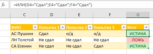
A simple OR operator determines whether the condition given in parentheses is met and returns one of the values TRUE or FALSE. In the future, this formula can be used as a component of more difficult conditions, when, depending on what will give the value OR, this or that action will be performed.
At the same time, they can be compared as numerical indicators, using the signs >,<, =, так и поиск конкретного значения для ячейки, которое может быть текстовым. В частности, для поиска слова «Сдал» в конкретных ячейках будет использоваться формула =ИЛИ(D4= “Сдал”; E4= “Сдал”; F4= “Сдал”)
Application: One way to use this function could be to take into account the success of passing the test of three attempts, where one pass is enough for further training / participation.
Finding and Using a Value
Horizontally
Using the HLOOKUP function, we can set a search for a specific table row, and at the output get a value from another cell in the same column (one or more rows lower), which corresponds to the specified condition. Moreover, the search is set either to the exact value (using the FALSE operator), or to the approximate value (with the TRUE operator), which allows the use of intervals. Syntax =HLOOKUP(lookup_value, table, row_number, interval_lookup)
Application: To calculate the bonus for a specific employee, you can set intervals, starting from which one or another percentage of profit is valid. Let's say the formula =GLOOKUP(E5;$D$1:$G$2;2;TRUE) will look in the first row of the table from the interval D1:G2 for a value approximately similar to the value from cell E5, and the result of the formula will be the output of the cell from the second row corresponding column.

Vertically
The VLOOKUP function works in a similar way - only the logic of the action is slightly different. The search will be carried out not horizontally, but vertically, that is, along the cells of one column, and the result will be taken from the specified cell of the found row.
That is, for the formula =VLOOKUP(E4;$I$3:$J$6;2;TRUE), the value of cell E4 will be compared with the cells of column I from the interval table I3:J6, and the value will be returned from the adjacent cell of column J.

Fulfillment of the IF condition
When using this function, a specific condition is specified, and then two results - one for cases where the conditions are met, and the other - vice versa. Let's say to compare funds from two columns, the following formula can be used =IF(C2>B2; “Over budget”; “Within budget”).
In addition, another function can be used as a condition, such as an OR condition and even another IF condition. At the same time, the IF functions can have from 3 to 64 possible results). As an example, =IF(D4=1, “YES”, IF(D4=2, “No”, “Maybe”)).
As a result, the value of the specified cell can also be displayed, both text and numeric. In this case, in the future it will be enough to change the value of one cell, without having to edit the formula in all places of use.

Ranking Formula
For the value of numbers, you can use the RANK formula, which will give the value of each number relative to others in a given list. In this case, the ranking can be both from a lower value towards an increase, and vice versa.
For the security of your documents, it is not superfluous to set a personal password on them.
For this function, three parameters are used - directly a number, an array or a reference to a list of numbers and order. In this case, if the order is not specified or the value is 0, then the rank is determined in descending order. Any other value for order will sort the values in ascending order.
Application: For a table with income by months, you can add a column with a ranking, and then sort by this column.

Maximum of selected values
A simple but very useful MAX formula gives highest value from a list of values. The list itself can consist of both cells and/or their range, as well as manually entered numbers. In total, the maximum value can be searched among a list of 255 numbers.
Application: Returning to the example with ranking, instead of the rank, you can display the value of the best indicator for the selected period.

Minimum of selected values
The search formula works in a similar way minimum values. Identical syntax, reverse output.

Average of selected values
There is also a formula to get the arithmetic mean from the selected list of values. However, its spelling in Russian is not so obvious. It sounds like AVERAGE, after which either specific values or cell references are indicated in brackets.

Sum of Selected Values
Finally, the most common feature that everyone who has ever used electronic Excel tables. Addition is performed using the SUM formula, and the interval or intervals of the cells whose values are to be summed are specified in brackets.
A much more interesting option is to sum the cells that meet specific criteria. To do this, use the SUMIF operator with arguments range, condition, summation range.
Application: For example, there is a list of schoolchildren who agreed to go on an excursion. Everyone has a status - whether he paid for the event or not. Thus, depending on the contents of the "Paid" column, the value from the "Cost" column will be considered or not. =SUMIF(E5:E9, "Yes", F5:F9)

Note: Detailed information on the use of each Excel functions can be found